Long before the advent of digital electronic technology, computers were built to electronically perform calculations by employing voltages and currents to represent numerical quantities. This was especially useful for the simulation of physical processes. A variable voltage, for instance, might represent velocity or force in a physical system. Through the use of resistive voltage dividers and voltage amplifiers, the mathematical operations of division and multiplication could be easily performed on these signals.
The reactive properties of capacitors and inductors lend themselves well to the simulation of variables related by calculus functions. Remember how the current through a capacitor was a function of the voltage's rate of change, and how that rate of change was designated in calculus as the derivative? Well, if voltage across a capacitor were made to represent the velocity of an object, the current through the capacitor would represent the force required to accelerate or decelerate that object, the capacitor's capacitance representing the object's mass:

This analog electronic computation of the calculus derivative function is technically known as differentiation, and it is a natural function of a capacitor's current in relation to the voltage applied across it. Note that this circuit requires no "programming" to perform this relatively advanced mathematical function as a digital computer would.
Electronic circuits are very easy and inexpensive to create compared to complex physical systems, so this kind of analog electronic simulation was widely used in the research and development of mechanical systems. For realistic simulation, though, amplifier circuits of high accuracy and easy configurability were needed in these early computers.
It was found in the course of analog computer design that differential amplifiers with extremely high voltage gains met these requirements of accuracy and configurability better than single-ended amplifiers with custom-designed gains. Using simple components connected to the inputs and output of the high-gain differential amplifier, virtually any gain and any function could be obtained from the circuit, overall, without adjusting or modifying the internal circuitry of the amplifier itself. These high-gain differential amplifiers came to be known as operational amplifiers, or op-amps, because of their application in analog computers' mathematical operations.
Modern op-amps, like the popular model 741, are high-performance, inexpensive integrated circuits. Their input impedances are quite high, the inputs drawing currents in the range of half a microamp (maximum) for the 741, and far less for op-amps utilizing field-effect input transistors. Output impedance is typically quite low, about 75 Ω for the model 741, and many models have built-in output short circuit protection, meaning that their outputs can be directly shorted to ground without causing harm to the internal circuitry. With direct coupling between op-amps' internal transistor stages, they can amplify DC signals just as well as AC (up to certain maximum voltage-risetime limits). It would cost far more in money and time to design a comparable discrete-transistor amplifier circuit to match that kind of performance, unless high power capability was required. For these reasons, op-amps have all but obsoleted discrete-transistor signal amplifiers in many applications.
The following diagram shows the pin connections for single op-amps (741 included) when housed in an 8-pin DIP (Dual Inline Package) integrated circuit:
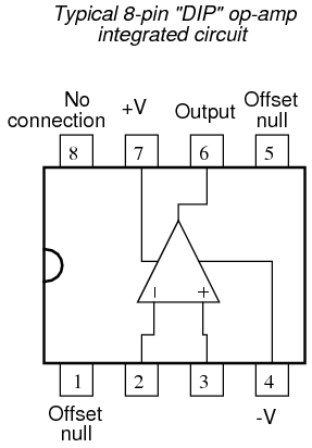
Some models of op-amp come two to a package, including the popular models TL082 and 1458. These are called "dual" units, and are typically housed in an 8-pin DIP package as well, with the following pin connections:

Operational amplifiers are also available four to a package, usually in 14-pin DIP arrangements. Unfortunately, pin assignments aren't as standard for these "quad" op-amps as they are for the "dual" or single units. Consult the manufacturer datasheet(s) for details.
Practical operational amplifier voltage gains are in the range of 200,000 or more, which makes them almost useless as an analog differential amplifier by themselves. For an op-amp with a voltage gain (AV) of 200,000 and a maximum output voltage swing of +15V/-15V, all it would take is a differential input voltage of 75 µV (microvolts) to drive it to saturation or cutoff! Before we take a look at how external components are used to bring the gain down to a reasonable level, let's investigate applications for the "bare" op-amp by itself.
One application is called the comparator. For all practical purposes, we can say that the output of an op-amp will be saturated fully positive if the (+) input is more positive than the (-) input, and saturated fully negative if the (+) input is less positive than the (-) input. In other words, an op-amp's extremely high voltage gain makes it useful as a device to compare two voltages and change output voltage states when one input exceeds the other in magnitude.
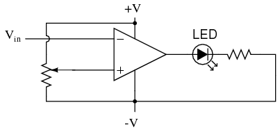
In the above circuit, we have an op-amp connected as a comparator, comparing the input voltage with a reference voltage set by the potentiometer (R1). If Vin drops below the voltage set by R1, the op-amp's output will saturate to +V, thereby lighting up the LED. Otherwise, if Vin is above the reference voltage, the LED will remain off. If Vin is a voltage signal produced by a measuring instrument, this comparator circuit could function as a "low" alarm, with the trip-point set by R1. Instead of an LED, the op-amp output could drive a relay, a transistor, an SCR, or any other device capable of switching power to a load such as a solenoid valve, to take action in the event of a low alarm.
Another application for the comparator circuit shown is a square-wave converter. Suppose that the input voltage applied to the inverting (-) input was an AC sine wave rather than a stable DC voltage. In that case, the output voltage would transition between opposing states of saturation whenever the input voltage was equal to the reference voltage produced by the potentiometer. The result would be a square wave:

Adjustments to the potentiometer setting would change the reference voltage applied to the noninverting (+) input, which would change the points at which the sine wave would cross, changing the on/off times, or duty cycle of the square wave:

It should be evident that the AC input voltage would not have to be a sine wave in particular for this circuit to perform the same function. The input voltage could be a triangle wave, sawtooth wave, or any other sort of wave that ramped smoothly from positive to negative to positive again. This sort of comparator circuit is very useful for creating square waves of varying duty cycle. This technique is sometimes referred to as pulse-width modulation, or PWM (varying, or modulating a waveform according to a controlling signal, in this case the signal produced by the potentiometer).
Another comparator application is that of the bargraph driver. If we had several op-amps connected as comparators, each with its own reference voltage connected to the inverting input, but each one monitoring the same voltage signal on their noninverting inputs, we could build a bargraph-style meter such as what is commonly seen on the face of stereo tuners and graphic equalizers. As the signal voltage (representing radio signal strength or audio sound level) increased, each comparator would "turn on" in sequence and send power to its respective LED. With each comparator switching "on" at a different level of audio sound, the number of LED's illuminated would indicate how strong the signal was.

In the circuit shown above, LED1 would be the first to light up as the input voltage increased in a positive direction. As the input voltage continued to increase, the other LED's would illuminate in succession, until all were lit.
This very same technology is used in some analog-to-digital signal converters, namely the flash converter, to translate an analog signal quantity into a series of on/off voltages representing a digital number.
The reactive properties of capacitors and inductors lend themselves well to the simulation of variables related by calculus functions. Remember how the current through a capacitor was a function of the voltage's rate of change, and how that rate of change was designated in calculus as the derivative? Well, if voltage across a capacitor were made to represent the velocity of an object, the current through the capacitor would represent the force required to accelerate or decelerate that object, the capacitor's capacitance representing the object's mass:
This analog electronic computation of the calculus derivative function is technically known as differentiation, and it is a natural function of a capacitor's current in relation to the voltage applied across it. Note that this circuit requires no "programming" to perform this relatively advanced mathematical function as a digital computer would.
Electronic circuits are very easy and inexpensive to create compared to complex physical systems, so this kind of analog electronic simulation was widely used in the research and development of mechanical systems. For realistic simulation, though, amplifier circuits of high accuracy and easy configurability were needed in these early computers.
It was found in the course of analog computer design that differential amplifiers with extremely high voltage gains met these requirements of accuracy and configurability better than single-ended amplifiers with custom-designed gains. Using simple components connected to the inputs and output of the high-gain differential amplifier, virtually any gain and any function could be obtained from the circuit, overall, without adjusting or modifying the internal circuitry of the amplifier itself. These high-gain differential amplifiers came to be known as operational amplifiers, or op-amps, because of their application in analog computers' mathematical operations.
Modern op-amps, like the popular model 741, are high-performance, inexpensive integrated circuits. Their input impedances are quite high, the inputs drawing currents in the range of half a microamp (maximum) for the 741, and far less for op-amps utilizing field-effect input transistors. Output impedance is typically quite low, about 75 Ω for the model 741, and many models have built-in output short circuit protection, meaning that their outputs can be directly shorted to ground without causing harm to the internal circuitry. With direct coupling between op-amps' internal transistor stages, they can amplify DC signals just as well as AC (up to certain maximum voltage-risetime limits). It would cost far more in money and time to design a comparable discrete-transistor amplifier circuit to match that kind of performance, unless high power capability was required. For these reasons, op-amps have all but obsoleted discrete-transistor signal amplifiers in many applications.
The following diagram shows the pin connections for single op-amps (741 included) when housed in an 8-pin DIP (Dual Inline Package) integrated circuit:
Some models of op-amp come two to a package, including the popular models TL082 and 1458. These are called "dual" units, and are typically housed in an 8-pin DIP package as well, with the following pin connections:
Operational amplifiers are also available four to a package, usually in 14-pin DIP arrangements. Unfortunately, pin assignments aren't as standard for these "quad" op-amps as they are for the "dual" or single units. Consult the manufacturer datasheet(s) for details.
Practical operational amplifier voltage gains are in the range of 200,000 or more, which makes them almost useless as an analog differential amplifier by themselves. For an op-amp with a voltage gain (AV) of 200,000 and a maximum output voltage swing of +15V/-15V, all it would take is a differential input voltage of 75 µV (microvolts) to drive it to saturation or cutoff! Before we take a look at how external components are used to bring the gain down to a reasonable level, let's investigate applications for the "bare" op-amp by itself.
One application is called the comparator. For all practical purposes, we can say that the output of an op-amp will be saturated fully positive if the (+) input is more positive than the (-) input, and saturated fully negative if the (+) input is less positive than the (-) input. In other words, an op-amp's extremely high voltage gain makes it useful as a device to compare two voltages and change output voltage states when one input exceeds the other in magnitude.
In the above circuit, we have an op-amp connected as a comparator, comparing the input voltage with a reference voltage set by the potentiometer (R1). If Vin drops below the voltage set by R1, the op-amp's output will saturate to +V, thereby lighting up the LED. Otherwise, if Vin is above the reference voltage, the LED will remain off. If Vin is a voltage signal produced by a measuring instrument, this comparator circuit could function as a "low" alarm, with the trip-point set by R1. Instead of an LED, the op-amp output could drive a relay, a transistor, an SCR, or any other device capable of switching power to a load such as a solenoid valve, to take action in the event of a low alarm.
Another application for the comparator circuit shown is a square-wave converter. Suppose that the input voltage applied to the inverting (-) input was an AC sine wave rather than a stable DC voltage. In that case, the output voltage would transition between opposing states of saturation whenever the input voltage was equal to the reference voltage produced by the potentiometer. The result would be a square wave:
Adjustments to the potentiometer setting would change the reference voltage applied to the noninverting (+) input, which would change the points at which the sine wave would cross, changing the on/off times, or duty cycle of the square wave:
It should be evident that the AC input voltage would not have to be a sine wave in particular for this circuit to perform the same function. The input voltage could be a triangle wave, sawtooth wave, or any other sort of wave that ramped smoothly from positive to negative to positive again. This sort of comparator circuit is very useful for creating square waves of varying duty cycle. This technique is sometimes referred to as pulse-width modulation, or PWM (varying, or modulating a waveform according to a controlling signal, in this case the signal produced by the potentiometer).
Another comparator application is that of the bargraph driver. If we had several op-amps connected as comparators, each with its own reference voltage connected to the inverting input, but each one monitoring the same voltage signal on their noninverting inputs, we could build a bargraph-style meter such as what is commonly seen on the face of stereo tuners and graphic equalizers. As the signal voltage (representing radio signal strength or audio sound level) increased, each comparator would "turn on" in sequence and send power to its respective LED. With each comparator switching "on" at a different level of audio sound, the number of LED's illuminated would indicate how strong the signal was.
In the circuit shown above, LED1 would be the first to light up as the input voltage increased in a positive direction. As the input voltage continued to increase, the other LED's would illuminate in succession, until all were lit.
This very same technology is used in some analog-to-digital signal converters, namely the flash converter, to translate an analog signal quantity into a series of on/off voltages representing a digital number.
- REVIEW:
- A triangle shape is the generic symbol for an amplifier circuit, the wide end signifying the input and the narrow end signifying the output.
- Unless otherwise specified, all voltages in amplifier circuits are referenced to a common ground point, usually connected to one terminal of the power supply. This way, we can speak of a certain amount of voltage being "on" a single wire, while realizing that voltage is always measured between two points.
- A differential amplifier is one amplifying the voltage difference between two signal inputs. In such a circuit, one input tends to drive the output voltage to the same polarity of the input signal, while the other input does just the opposite. Consequently, the first input is called the noninverting (+) input and the second is called the inverting (-) input.
- An operational amplifier (or op-amp for short) is a differential amplifier with an extremely high voltage gain (AV = 200,000 or more). Its name hails from its original use in analog computer circuitry (performing mathematical operations).
- Op-amps typically have very high input impedances and fairly low output impedances.
- Sometimes op-amps are used as signal comparators, operating in full cutoff or saturation mode depending on which input (inverting or noninverting) has the greatest voltage. Comparators are useful in detecting "greater-than" signal conditions (comparing one to the other).
- One comparator application is called the pulse-width modulator, and is made by comparing a sine-wave AC signal against a DC reference voltage. As the DC reference voltage is adjusted, the square-wave output of the comparator changes its duty cycle (positive versus negative times). Thus, the DC reference voltage controls, or modulates the pulse width of the output voltage.


