The branch of physics that deals with the action of forces on matter is referred to as mechanics. All considerations of motion are addressed by mechanics, as well as the transmission of forces through the use of simple machines. In our class, the goal is a mechanical goal (placing blocks into a bin) and electronics are used to control the mechanics.
While it is not necessary to sit down and draw free body diagrams or figure out the static coefficient of friction between the LEGO tires and the game board, it is helpful to keep certain mechanical concepts in mind when constructing a robot. If a robot's tires are spinning because they do not grip the floor, then something must be done to increase the friction between the tires and the floor. One solution is to glue a rubber band around the circumference of the tire. That problem/solution did not require an in-depth study of physics. Simply considering the different possibilities can lead to more mechanically creative robots.
Describing motion involves more than just saying that an object moved three feet to the right. The magnitude and direction of the displacement are important, but so are the characteristics of the object's velocity and acceleration. To understand these concepts, we must examine the nature of force. Changes in the motion of an object are created by forces.
Click here to read more about basic mechanics and its principals.
Monday, December 27, 2010
Holography
Holography

The above image was taken through a transmission hologram. The hologram was illuminated from behind by a helium-neon laser which has been passed through a diverging lens to spread the beam over the hologram.
Holography is "lensless photography" in which an image is captured not as an image focused on film, but as an interference pattern at the film. Typically, coherent light from a laser is reflected from an object and combined at the film with light from a reference beam. This recorded interference pattern actually contains much more information that a focused image, and enables the viewer to view a true three-dimensional image which exhibits parallax. That is, the image will change its appearance if you look at it from a different angle, just as if you were looking at a real 3D object. In the case of a transmission hologram, you look through the film and see the three dimensional image suspended in midair at a point which corresponds to the position of the real object which was photographed.


These three images of the same hologram were taken by positioning the camera at three positions, moving from left to right. Note that the pawn appears on the left side of the king in the left photo, but transitions to the right of the king as you sweep your eye across the hologram. This is real parallax, which tells you that the image is truly 3-dimensional. Each perspective corresponds to looking through the hologram at a particular point.
The Holographic Image
Some of the descriptions of holograms are
Some of the descriptions of holograms are
"image formation by wavefront reconstruction.."
"lensless photography"
"freezing an image on its way to your eye, and then reconstructing it with a laser"
A consistent characteristic of the images as viewed
The images are true three-dimensional images, showing depth and parallax and continually changing in aspect with the viewing angle.
Any part of the hologram contains the whole image!
The images are scalable. They can be made with one wavelength and viewed with another, with the possibility of magnification.
Friday, December 24, 2010
Super Conductivity
If mercury is cooled below 4.1 K, it loses all electric resistance. This discovery of superconductivity by H. Kammerlingh Onnes in 1911 was followed by the observation of other metals which exhibit zero resistivity below a certain critical temperature. The fact that the resistance is zero has been demonstrated by sustaining currents in superconducting lead rings for many years with no measurable reduction. An induced current in an ordinary metal ring would decay rapidly from the dissipation of ordinary resistance, but superconducting rings had exhibited a decay constant of over a billion years!
Meissner effect:
When a material makes the transition from the normal to superconducting state, it actively excludes magnetic fields from its interior; this is called the Meissner effect.
This constraint to zero magnetic field inside a superconductor is distinct from the perfect diamagnetism which would arise from its zero electrical resistance. Zero resistance would imply that if you tried to magnetize a superconductor, current loops would be generated to exactly cancel the imposed field (Lenz's law). But if the material already had a steady magnetic field through it when it was cooled trough the superconducting transition, the magnetic field would be expected to remain. If there were no change in the applied magnetic field, there would be no generated voltage (Faraday's law) to drive currents, even in a perfect conductor. Hence the active exclusion of magnetic field must be considered to be an effect distinct from just zero resistance. A mixed state Meissner effect occurs with Type II materials.
Perfect Diamagnet
If a conductor already had a steady magnetic field through it and was then cooled through the transition to a zero resistance state, becoming a perfect diamagnet, the magnetic field would be expected to stay the same.
 Superconductor
Remarkably, the magnetic behavior of a superconductor is distinct from perfect diamagnetism. It will actively exclude any magnetic field present when it makes the phase change to the superconducting state.

BCS Theory of Superconductivity:
The properties of Type I superconductors were modeled successfully by the efforts of John Bardeen, Leon Cooper, and Robert Schrieffer in what is commonly called the BCS theory. A key conceptual element in this theory is the pairing of electrons close to the Fermi level into Cooper pairs through interaction with the crystal lattice. This pairing results from a slight attraction between the electrons related to lattice vibrations; the coupling to the lattice is called a phonon interaction.
Pairs of electrons can behave very differently from single electrons which are fermions and must obey the Pauli exclusion principle. The pairs of electrons act more like bosons which can condense into the same energy level. The electron pairs have a slightly lower energy and leave an energy gap above them on the order of .001 eV which inhibits the kind of collision interactions which lead to ordinary resistivity. For temperatures such that the thermal energy is less than the band gap, the material exhibits zero resistivity.
Bardeen, Cooper, and Schrieffer received the Nobel Prize in 1972 for the development of the theory of superconductivity.
I want to know the BCS Theory deeply
Cooper Pairs:

The behavior of superconductors suggests that electron pairs are coupling over a range of hundreds of nanometers, three orders of magnitude larger than the lattice spacing. Called Cooper pairs, these coupled electrons can take the character of a boson and condense into the ground state.
This pair condensation is the basis for the BCS theory of superconductivity. The effective net attraction between the normally repulsive electrons produces a pair binding energy on the order of milli-electron volts, enough to keep them paired at extremely low temperatures.
Isotope Effect, Mercury
If electrical conduction in mercury were purely electronic, there should be no dependence upon the nuclear masses. This dependence of the critical temperature for superconductivity upon isotopic mass was the first direct evidence for interaction between the electrons and the lattice. This supported the BCS theory of lattice coupling of electron pairs.
It is quite remarkable that an electrical phenomenon like the transition to zero resistivity should involve a purely mechanical property of the lattice. Since a change in the critical temperature involves a change in the energy environment associated with the superconducting transition, this suggests that part of the energy is being used to move the atoms of the lattice since the energy depends upon the mass of the lattice. This indicates that lattice vibrations are a part of the superconducting process. This was an important clue in the process of developing the BCS theory because it suggested lattice coupling, and in the quantum treatment suggested that phonons were involved.
Type I Superconductors:
The thirty pure metals listed at right below are called Type I superconductors. The identifying characteristics are zero electrical resistivity below a critical temperature, zero internal magnetic field (Meissner effect), and a critical magnetic field above which superconductivity ceases.
The superconductivity in Type I superconductors is modeled well by the BCS theory which relies upon electron pairs coupled by lattice vibration interactions. Remarkably, the best conductors at room temperature (gold, silver, and copper) do not become superconducting at all. They have the smallest lattice vibrations, so their behavior correlates well with the BCS Theory.
While instructive for understanding superconductivity, the Type I superconductors have been of limited practical usefulness because the critical magnetic fields are so small and the superconducting state disappears suddenly at that temperature. Type I superconductors are sometimes called "soft" superconductors while the Type II are "hard", maintaining the superconducting state to higher temperatures and magnetic fields.
Type II Superconductors:
Superconductors made from alloys are called Type II superconductors. Besides being mechanically harder than Type I superconductors, they exhibit much higher critical magnetic fields. Type II superconductors such as niobium-titanium (NbTi) are used in the construction of high field superconducting magnets.
Type-II superconductors usually exist in a mixed state of normal and superconducting regions. This is sometimes called a vortex state, because vortices of superconducting currents surround filaments or cores of normal material.
Meissner effect:
When a material makes the transition from the normal to superconducting state, it actively excludes magnetic fields from its interior; this is called the Meissner effect.
This constraint to zero magnetic field inside a superconductor is distinct from the perfect diamagnetism which would arise from its zero electrical resistance. Zero resistance would imply that if you tried to magnetize a superconductor, current loops would be generated to exactly cancel the imposed field (Lenz's law). But if the material already had a steady magnetic field through it when it was cooled trough the superconducting transition, the magnetic field would be expected to remain. If there were no change in the applied magnetic field, there would be no generated voltage (Faraday's law) to drive currents, even in a perfect conductor. Hence the active exclusion of magnetic field must be considered to be an effect distinct from just zero resistance. A mixed state Meissner effect occurs with Type II materials.
Perfect Diamagnet
If a conductor already had a steady magnetic field through it and was then cooled through the transition to a zero resistance state, becoming a perfect diamagnet, the magnetic field would be expected to stay the same.
Remarkably, the magnetic behavior of a superconductor is distinct from perfect diamagnetism. It will actively exclude any magnetic field present when it makes the phase change to the superconducting state.
BCS Theory of Superconductivity:
The properties of Type I superconductors were modeled successfully by the efforts of John Bardeen, Leon Cooper, and Robert Schrieffer in what is commonly called the BCS theory. A key conceptual element in this theory is the pairing of electrons close to the Fermi level into Cooper pairs through interaction with the crystal lattice. This pairing results from a slight attraction between the electrons related to lattice vibrations; the coupling to the lattice is called a phonon interaction.
Pairs of electrons can behave very differently from single electrons which are fermions and must obey the Pauli exclusion principle. The pairs of electrons act more like bosons which can condense into the same energy level. The electron pairs have a slightly lower energy and leave an energy gap above them on the order of .001 eV which inhibits the kind of collision interactions which lead to ordinary resistivity. For temperatures such that the thermal energy is less than the band gap, the material exhibits zero resistivity.
Bardeen, Cooper, and Schrieffer received the Nobel Prize in 1972 for the development of the theory of superconductivity.
I want to know the BCS Theory deeply
Cooper Pairs:
The behavior of superconductors suggests that electron pairs are coupling over a range of hundreds of nanometers, three orders of magnitude larger than the lattice spacing. Called Cooper pairs, these coupled electrons can take the character of a boson and condense into the ground state.
This pair condensation is the basis for the BCS theory of superconductivity. The effective net attraction between the normally repulsive electrons produces a pair binding energy on the order of milli-electron volts, enough to keep them paired at extremely low temperatures.
Isotope Effect, Mercury
If electrical conduction in mercury were purely electronic, there should be no dependence upon the nuclear masses. This dependence of the critical temperature for superconductivity upon isotopic mass was the first direct evidence for interaction between the electrons and the lattice. This supported the BCS theory of lattice coupling of electron pairs.
It is quite remarkable that an electrical phenomenon like the transition to zero resistivity should involve a purely mechanical property of the lattice. Since a change in the critical temperature involves a change in the energy environment associated with the superconducting transition, this suggests that part of the energy is being used to move the atoms of the lattice since the energy depends upon the mass of the lattice. This indicates that lattice vibrations are a part of the superconducting process. This was an important clue in the process of developing the BCS theory because it suggested lattice coupling, and in the quantum treatment suggested that phonons were involved.
Type I Superconductors:
The thirty pure metals listed at right below are called Type I superconductors. The identifying characteristics are zero electrical resistivity below a critical temperature, zero internal magnetic field (Meissner effect), and a critical magnetic field above which superconductivity ceases.
The superconductivity in Type I superconductors is modeled well by the BCS theory which relies upon electron pairs coupled by lattice vibration interactions. Remarkably, the best conductors at room temperature (gold, silver, and copper) do not become superconducting at all. They have the smallest lattice vibrations, so their behavior correlates well with the BCS Theory.
While instructive for understanding superconductivity, the Type I superconductors have been of limited practical usefulness because the critical magnetic fields are so small and the superconducting state disappears suddenly at that temperature. Type I superconductors are sometimes called "soft" superconductors while the Type II are "hard", maintaining the superconducting state to higher temperatures and magnetic fields.
Type II Superconductors:
Superconductors made from alloys are called Type II superconductors. Besides being mechanically harder than Type I superconductors, they exhibit much higher critical magnetic fields. Type II superconductors such as niobium-titanium (NbTi) are used in the construction of high field superconducting magnets.
Type-II superconductors usually exist in a mixed state of normal and superconducting regions. This is sometimes called a vortex state, because vortices of superconducting currents surround filaments or cores of normal material.
Thursday, December 23, 2010
Refrigeration Cycle
- The compressor
- The condenser
- The expansion device
- The evaporator

The copper refrigerant tube (a tube that connects these air conditioner parts)
We’ll be discussing the refrigeration cycle from split-central air conditioner units perspective; to make it easier.
Remember: refrigeration is a process that removes heat from an area that is not wanted and transfers that heat to an area that meaningless.
Ok, lets get started.
In this refrigeration diagram, the four major components split into two sections: Indoor and Outdoor. In indoor units, we have the AC parts number 1 and 2. In outdoor units, we have the AC parts number 3 and 4.
These four majors’ components are divided into two difference pressure: high pressure and low pressure.
The high pressure side is the condenser units (outdoor) and the low pressure side is the air conditioning evaporator (indoor). The divided point between high and low pressure cut through the compressor and the expansion valve.
Refrigeration cycle is a process that removes heat from indoor evaporator to outdoor condenser units. How does it do that?
AC parts # 1, Air conditioner evaporator.
The air conditioning evaporator is a heat exchanger that absorbs heat into the air conditioner system. The evaporator does not exactly absorb heat! It’s the cooled refrigerant fed from the bottom of the evaporator coils absorb the heat.
The liquid refrigerant usually flows from the bottom of the evaporator coils and boils as it moves to the top of the evaporator coils.
The reason it’s fed from the bottom is to ensure the liquid refrigerant boils before it leave the evaporator coils.
If a refrigerant was to fed from the top, the liquid refrigerant would easily drop to the bottom of the coils before it absorbs enough heat and boil.
If evaporator was too feed liquid refrigerant into air conditioner compressor; it will shorts the air conditioner compressor life.
This how air conditioning evaporator boils liquid refrigerant to vapor.
A (40°F) refrigerant flows through the evaporator, it absorbs 75°F indoor heat, causing the liquid refrigerant in the evaporator to boils.
Side Notes* the temperature of the refrigerant will always try to equalize. The 75°F heat will flow to 40°F refrigerant and it will increases the 40°F temperature and boils it.
After the liquid refrigerant travel across the evaporator coils, the entire liquid refrigerant should have boils. At this point it’s known as saturated vapor point.
The air conditioner evaporator has three important tasks:
Its absorb heat
Boils all the refrigerant to vapor aka saturated vapor
Superheat
Air conditioner parts # 2, Air conditioner compressors.
The air conditioning compressor is known as the heart of the air conditioner units. It’s one of the divided points between high and low side.
As you can see in the refrigeration cycle diagram; the compressor has a refrigerant inlet line and refrigerant outlet line.
The compressor inlet lines are known as:
Suction pressure
Back pressure
Low side pressure
The compressor outlet lines are known as:
High side pressure
Discharge pressure
Head pressure
The compressor absorbs vapor refrigerant from the suction line and compresses that heat to high superheat vapor.
As the refrigerant flows across the compressor, it also removes heat of compression, motor winding heat, mechanical friction, and other heat absorbs in the suction line.
The air conditioner units compressor produce the pressure different, it’s the air conditioner compressors that cause the refrigerant to flow in a cycle.
The compressor is a VAPOR pump!
Air conditioner parts # 3, Air conditioner condenser .
In this refrigeration cycle diagram, the air conditioner condenser is air cooled condenser. It functions the same way as the evaporator but it does the opposite.
The condenser units are located outdoor with the compressor. It purposes is to reject both sensible and latent heat of vapor absorb by the air conditioner units.
The condenser receives high pressure and high temperature superheats vapor from the compressor and rejects that heat to the low temperature air. After rejected all the vapor heat, it turns back to liquid refrigerant.
The condenser has three important steps:
Its remove sensible heat or (de-superheat)
Remove latent heat or (condense)
Remove more sensible heat or (subcooled)
Air conditioner parts # 4, Air conditioner expansion valve or Thermostatic Expansion Valve (TXV’s) (TEV’s).
or Thermostatic Expansion Valve (TXV’s) (TEV’s).
All expansion device or metering device has similar function (to some extent); it’s responsible for providing the correct amount of refrigerant to the evaporator.
This is done by creating a restriction within the thermostatic expansion valve. The restriction causes the pressure and temperature of the refrigerant entering the Evaporator to reduce.
The refrigeration cycle diagram above has a thermostatic expansion valve. This expansion device has
Remote Bulb
Capillary Tube
TXV Body
Thermostatic expansion valve has other components besides these three. However, they are not important right now.
How does TXV provides the correct amount of refrigerant?
TXV provides the correct amount of air conditioner refrigerant to the evaporator by using a remote sensing bulb as a regulator. The remote sensing bulb and capillary tube has a refrigerant inside.
As you can see in the refrigeration cycle diagram above, the remote sensing bulb is tie with the suction line. The temperature from the suction line transfer heat to the sensing bulb through conduction.
Sensing bulb responds to the temperature of the suction line and as a result, it decreases or increases the temperature and pressure inside the sensing bulb due to suction line temperatures. The sensing bulb also has a diaphragm on the other end. This diaphragm is with the TXV body.
The diaphragm is the device that pushes or releases the needle from the valve seat. There is so much to it, but I hope this explains how expansion device work.
Remember* Refrigeration cycle diagram will always have the same basic components (compressor, condenser, expansion device, evaporator, and refrigerant tube.
These components may be in difference shape, capacity and size, but it does the same thing.
If you understand how the refrigeration cycle works, you understand how any air conditioner works. Since all air conditioners have the same basic five components and basic refrigeration cycle.
Saturday, October 23, 2010
Diodes And Rectifiers
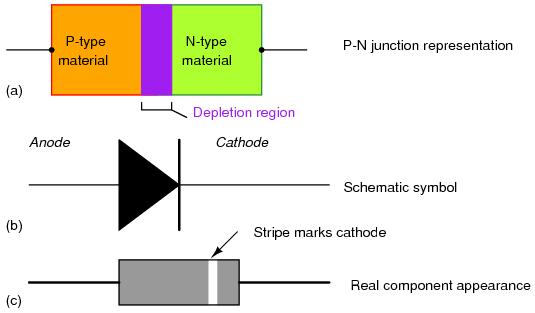
A diode is an electrical device allowing current to move through it in one direction with far greater ease than in the other. The most common kind of diode in modern circuit design is the semiconductor diode, although other diode technologies exist. Semiconductor diodes are symbolized in schematic diagrams such as Figure below. The term “diode” is customarily reserved for small signal devices, I ≤ 1 A. The term rectifier is used for power devices, I > 1 A.
Wednesday, October 13, 2010
Eigon Vectors
An eigen vector is a vector that is scaled by a linear transformation, but not moved. Think of an eigen vector as an arrow whose direction is not changed. It may stretch, or shrink, as space is transformed, but it continues to point in the same direction. Most arrows will move, as illustrated by a spinning planet, but some vectors will continue to point in the same direction, such as the north pole.
The scaling factor of an eigen vector is called its eigen value. An eigen value only makes sense in the context of an eigen vector, i.e. the arrow whose length is being changed.
In the plane, a rigid rotation of 90° has no eigen vectors, because all vectors move. However, the reflection y = -y has the x and y axes as eigen vectors. In this function, x is scaled by 1 and y by -1, the eigen values corresponding to the two eigen vectors. All other vectors move in the plane.
The y axis, in the above example, is subtle. The direction of the vector has been reversed, yet we still call it an eigen vector, because it lives in the same line as the original vector. It has been scaled by -1, pointing in the opposite direction. An eigen vector stretches, or shrinks, or reverses course, or squashes down to 0. The key is that the output vector is a constant (possibly negative) times the input vector.
These concepts are valid over a division ring, as well as a field. Multiply by K on the left to build the K vector space, and apply the transformation, as a matrix, on the right. However, the following method for deriving eigen values and vectors is based on the determinant, and requires a field.
If the eigen space is nontrivial then the determinant of Q must be 0. Expand the determinant, giving an n degree polynomial in l. (This is where we need a field, to pull all the entries to the left of l, and build a traditional polynomial.) This is called the characteristic polynomial of the matrix. The roots of this polynomial are the eigen values. There are at most n eigen values.
Substitute each root in turn and find the kernel of Q. We are looking for the set of vectors x such that x*Q = 0. Let R be the transpose of Q and solve R*x = 0, where x has become a column vector. This is a set of simultaneous equations that can be solved using gaussian elimination.
In summary, a somewhat straightforward algorithm extracts the eigen values, by solving an n degree polynomial, then derives the eigen space for each eigen value.
Some eigen values will produce multiple eigen vectors, i.e. an eigen space with more than one dimension. The identity matrix, for instance, has an eigen value of 1, and an n-dimensional eigen space to go with it. In contrast, an eigen value may have multiplicity > 1, yet there is only one eigen vector. This is illustrated by [1,1|0,1], a function that tilts the x axis counterclockwise and leaves the y axis alone. The eigen values are 1 and 1, and the eigen vector is 0,1, namely the y axis.
Select a basis b for the eigen space of l. The vectors in b are eigen vectors, with eigen value l, and every eigen vector with eigen value l is spanned by b. Conversely, an eigen vector with some other eigen value lies outside of b.
Let the first 7 vectors share a common eigen value l. If these vectors are dependent then one of them can be expressed as a linear combination of the other 6. Make this substitution and find a shorter list of dependent eigen vectors that do not all share the same eigen value. The first 6 have eigen value l, and the rest have some other eigen value. Remember, we selected the shortest list, so this is a contradiction. Therefore the eigen vectors associated with any given eigen value are independent.
Scale all the coefficients c1 through ck by a common factor s. This does not change the fact that the sum of cixi is still zero. However, other than this scaling factor, we will prove there are no other coefficients that carry the eigen vectors to 0.
If there are two independent sets of coefficients that lead to 0, scale them so the first coefficients in each set are equal, then subtract. This gives a shorter linear combination of dependent eigen vectors that yields 0. More than one vector remains, else cjxj = 0, and xj is the 0 vector. We already showed these dependent eigen vectors cannot share a common eigen value, else they would be linearly independent; thus multiple eigen values are represented. This is a shorter list of dependent eigen vectors with multiple eigen values, which is a contradiction.
If a set of coefficients carries our eigen vectors to 0, it must be a scale multiple of c1 c2 c3 … ck.
Now take the sum of cixi and multiply by M on the right. In other words, apply the linear transformation. The image of 0 ought to be 0. Yet each coefficient is effectively multiplied by the eigen value for its eigen vector, and not all eigen values are equal. In particular, not all eigen values are 0. The coefficients are not scaled equally. The new linear combination of eigen vectors is not a scale multiple of the original, and is not zero across the board. It represents a new way to combine eigen vectors to get 0. If there were two eigen values before, and one of them was zero, there is but one eigen value now. However, this means the vectors associated with that one eigen value are dependent, and we already ruled that out. Therefore we still have two or more eigen values represented. This cannot be a shorter list, so all eigen vectors are still present. In other words, all our original eigen values were nonzero. Hence a different linear combination of our eigen vectors yields 0, and that is impossible.
Therefore the eigen spaces produced by different eigen values are linearly independent.
These results, for eigen values and eigen vectors, are valid over a division ring.
The scaling factor of an eigen vector is called its eigen value. An eigen value only makes sense in the context of an eigen vector, i.e. the arrow whose length is being changed.
In the plane, a rigid rotation of 90° has no eigen vectors, because all vectors move. However, the reflection y = -y has the x and y axes as eigen vectors. In this function, x is scaled by 1 and y by -1, the eigen values corresponding to the two eigen vectors. All other vectors move in the plane.
The y axis, in the above example, is subtle. The direction of the vector has been reversed, yet we still call it an eigen vector, because it lives in the same line as the original vector. It has been scaled by -1, pointing in the opposite direction. An eigen vector stretches, or shrinks, or reverses course, or squashes down to 0. The key is that the output vector is a constant (possibly negative) times the input vector.
These concepts are valid over a division ring, as well as a field. Multiply by K on the left to build the K vector space, and apply the transformation, as a matrix, on the right. However, the following method for deriving eigen values and vectors is based on the determinant, and requires a field.
Finding Eigen Values and Vectors
Given a matrix M implementing a linear transformation, what are its eigen vectors and values? Let the vector x represent an eigen vector and let l be the eigen value. We must solve x*M = lx. Rewrite lx as x times l times the identity matrix and subtract it from both sides. The right side drops to 0, and the left side is x*M-x*l*identity. Pull x out of both factors and write x*Q = 0, where Q is M with l subtracted from the main diagonal. The eigen vector x lies in the kernel of the map implemented by Q. The entire kernel is known as the eigen space, and of course it depends on the value of l.If the eigen space is nontrivial then the determinant of Q must be 0. Expand the determinant, giving an n degree polynomial in l. (This is where we need a field, to pull all the entries to the left of l, and build a traditional polynomial.) This is called the characteristic polynomial of the matrix. The roots of this polynomial are the eigen values. There are at most n eigen values.
Substitute each root in turn and find the kernel of Q. We are looking for the set of vectors x such that x*Q = 0. Let R be the transpose of Q and solve R*x = 0, where x has become a column vector. This is a set of simultaneous equations that can be solved using gaussian elimination.
In summary, a somewhat straightforward algorithm extracts the eigen values, by solving an n degree polynomial, then derives the eigen space for each eigen value.
Some eigen values will produce multiple eigen vectors, i.e. an eigen space with more than one dimension. The identity matrix, for instance, has an eigen value of 1, and an n-dimensional eigen space to go with it. In contrast, an eigen value may have multiplicity > 1, yet there is only one eigen vector. This is illustrated by [1,1|0,1], a function that tilts the x axis counterclockwise and leaves the y axis alone. The eigen values are 1 and 1, and the eigen vector is 0,1, namely the y axis.
The Same Eigen Value
Let two eigen vectors have the same eigen value. specifically, let a linear map multiply the vectors v and w by the scaling factor l. By linearity, 3v+4w is also scaled by l. In fact every linear combination of v and w is scaled by l. When a set of vectors has a common eigen value, the entire space spanned by those vectors is an eigen space, with the same eigen value. This is not surprising, since the eigen vectors associated with l are precisely the kernel of the transfoormation defined by the matrix M with l subtracted from the main diagonal. This kernel is a vector space, and so is the eigen space of l.Select a basis b for the eigen space of l. The vectors in b are eigen vectors, with eigen value l, and every eigen vector with eigen value l is spanned by b. Conversely, an eigen vector with some other eigen value lies outside of b.
Different Eigen Values
Different eigen values always lead to independent eigen spaces. Suppose we have the shortest counterexample. Thus c1x1 + c2x2 + … + ckxk = 0. Here x1 through xk are the eigen vectors, and c1 through ck are the coefficients that prove the vectors form a dependent set. Furthermore, the vectors represent at least two different eigen values.Let the first 7 vectors share a common eigen value l. If these vectors are dependent then one of them can be expressed as a linear combination of the other 6. Make this substitution and find a shorter list of dependent eigen vectors that do not all share the same eigen value. The first 6 have eigen value l, and the rest have some other eigen value. Remember, we selected the shortest list, so this is a contradiction. Therefore the eigen vectors associated with any given eigen value are independent.
Scale all the coefficients c1 through ck by a common factor s. This does not change the fact that the sum of cixi is still zero. However, other than this scaling factor, we will prove there are no other coefficients that carry the eigen vectors to 0.
If there are two independent sets of coefficients that lead to 0, scale them so the first coefficients in each set are equal, then subtract. This gives a shorter linear combination of dependent eigen vectors that yields 0. More than one vector remains, else cjxj = 0, and xj is the 0 vector. We already showed these dependent eigen vectors cannot share a common eigen value, else they would be linearly independent; thus multiple eigen values are represented. This is a shorter list of dependent eigen vectors with multiple eigen values, which is a contradiction.
If a set of coefficients carries our eigen vectors to 0, it must be a scale multiple of c1 c2 c3 … ck.
Now take the sum of cixi and multiply by M on the right. In other words, apply the linear transformation. The image of 0 ought to be 0. Yet each coefficient is effectively multiplied by the eigen value for its eigen vector, and not all eigen values are equal. In particular, not all eigen values are 0. The coefficients are not scaled equally. The new linear combination of eigen vectors is not a scale multiple of the original, and is not zero across the board. It represents a new way to combine eigen vectors to get 0. If there were two eigen values before, and one of them was zero, there is but one eigen value now. However, this means the vectors associated with that one eigen value are dependent, and we already ruled that out. Therefore we still have two or more eigen values represented. This cannot be a shorter list, so all eigen vectors are still present. In other words, all our original eigen values were nonzero. Hence a different linear combination of our eigen vectors yields 0, and that is impossible.
Therefore the eigen spaces produced by different eigen values are linearly independent.
These results, for eigen values and eigen vectors, are valid over a division ring.
Axis of Rotation
Here is a simple application of eigen vectors. A rigid rotation in 3 space always has an axis of rotation. Let M implement the rotation. The determinant of M, with l subtracted from its main diagonal, gives a cubic polynomial in l, and every cubic has at least one real root. Since lengths are preserved by a rotation, l is ±1. If l is -1 we have a reflection. So l = 1, and the space rotates through some angle θ about the eigen vector. That's why every planet, every star, has an axis of rotation.Wednesday, October 6, 2010
Lasers
A laser is constructed from three principal parts:

The pump source is the part that provides energy to the laser system. Examples of pump sources include electrical discharges, flashlamps, arc lamps, light from another laser, chemical reactions and even explosive devices. The type of pump source used principally depends on the gain medium, and this also determines how the energy is transmitted to the medium. A helium-neon (HeNe) laser uses an electrical discharge in the helium-neon gas mixture, a Nd:YAG laser uses either light focused from a xenon flash lamp or diode lasers, and excimer lasers use a chemical reaction.laser is not only light source
The gain medium is the major determining factor of the wavelength of operation, and other properties, of the laser.Gain media in different materials have linear spectra or wide spectra.Gain media with wide spectra allow tune frequency of laser.First wide tunable crystal laser with tunabulity more octave represent on photo 3 http://spie.org/x39922.xml . There are hundreds if thousands of different gain media in which laser operation has been achieved (see list of laser types for a list of the most important ones). The gain medium is excited by the pump source to produce a population inversion, and it is in the gain medium that spontaneous and stimulated emission of photons takes place, leading to the phenomenon of optical gain, or amplification.
Examples of different gain media include:
The optical resonator, or optical cavity, in its simplest form is two parallel mirrors placed around the gain medium which provide feedback of the light. The mirrors are given optical coatings which determine their reflective properties. Typically one will be a high reflector, and the other will be a partial reflector. The latter is called the output coupler, because it allows some of the light to leave the cavity to produce the laser's output beam.
Light from the medium, produced by spontaneous emission, is reflected by the mirrors back into the medium, where it may be amplified by stimulated emission. The light may reflect from the mirrors and thus pass through the gain medium many hundreds of times before exiting the cavity. In more complex lasers, configurations with four or more mirrors forming the cavity are used. The design and alignment of the mirrors with respect to the medium is crucial to determining the exact operating wavelength and other attributes of the laser system.
Other optical devices, such as spinning mirrors, modulators, filters, and absorbers, may be placed within the optical resonator to produce a variety of effects on the laser output, such as altering the wavelength of operation or the production of pulses of laser light.
Some lasers do not use an optical cavity, but instead rely on very high optical gain to produce significant amplified spontaneous emission (ASE) without needing feedback of the light back into the gain medium. Such lasers are said to be superluminescent, and emit light with low coherence but high bandwidth. Since they do not use optical feedback, these devices are often not categorized as lasers.
Q-switching, sometimes known as giant pulse formation, is a technique by which a laser can be made to produce a pulsed output beam. The technique allows the production of light pulses with extremely high (gigawatt) peak power, much higher than would be produced by the same laser if it were operating in a continuous wave (constant output) mode. Compared to modelocking, another technique for pulse generation with lasers, Q-switching leads to much lower pulse repetition rates, much higher pulse energies, and much longer pulse durations. Both techniques are sometimes applied at once.
Initially the laser medium is pumped while the Q-switch is set to prevent feedback of light into the gain medium (producing an optical resonator with low Q). This produces a population inversion, but laser operation cannot yet occur since there is no feedback from the resonator. Since the rate of stimulated emission is dependent on the amount of light entering the medium, the amount of energy stored in the gain medium increases as the medium is pumped. Due to losses from spontaneous emission and other processes, after a certain time the stored energy will reach some maximum level; the medium is said to be gain saturated. At this point, the Q-switch device is quickly changed from low to high Q, allowing feedback and the process of optical amplification by stimulated emission to begin. Because of the large amount of energy already stored in the gain medium, the intensity of light in the laser resonator builds up very quickly; this also causes the energy stored in the medium to be depleted almost as quickly. The net result is a short pulse of light output from the laser, known as a giant pulse, which may have a very high peak intensity.
- An energy source (usually referred to as the pump or pump source),
- A gain medium or laser medium, and
- Two or more mirrors that form an optical resonator.

Pump source
The pump source is the part that provides energy to the laser system. Examples of pump sources include electrical discharges, flashlamps, arc lamps, light from another laser, chemical reactions and even explosive devices. The type of pump source used principally depends on the gain medium, and this also determines how the energy is transmitted to the medium. A helium-neon (HeNe) laser uses an electrical discharge in the helium-neon gas mixture, a Nd:YAG laser uses either light focused from a xenon flash lamp or diode lasers, and excimer lasers use a chemical reaction.laser is not only light source
Gain medium / Laser medium
The gain medium is the major determining factor of the wavelength of operation, and other properties, of the laser.Gain media in different materials have linear spectra or wide spectra.Gain media with wide spectra allow tune frequency of laser.First wide tunable crystal laser with tunabulity more octave represent on photo 3 http://spie.org/x39922.xml . There are hundreds if thousands of different gain media in which laser operation has been achieved (see list of laser types for a list of the most important ones). The gain medium is excited by the pump source to produce a population inversion, and it is in the gain medium that spontaneous and stimulated emission of photons takes place, leading to the phenomenon of optical gain, or amplification.
Examples of different gain media include:
- Liquids, such as dye lasers. These are usually organic chemical solvents, such as methanol, ethanol or ethylene glycol, to which are added chemical dyes such as coumarin, rhodamine and fluorescein. The exact chemical configuration of the dye molecules determines the operation wavelength of the dye laser.
- Gases, such as carbon dioxide, argon, krypton and mixtures such as helium-neon. These lasers are often pumped by electrical discharge.
- Solids, such as crystals and glasses. The solid host materials are usually doped with an impurity such as chromium, neodymium, erbium or titanium ions. Typical hosts include YAG (yttrium aluminium garnet), YLF (yttrium lithium fluoride), sapphire (aluminium oxide) and various glasses. Examples of solid-state laser media include Nd:YAG, Ti:sapphire, Cr:sapphire (usually known as ruby), Cr:LiSAF (chromium-doped lithium strontium aluminium fluoride), Er:YLF, Nd:glass, and Er:glass. Solid-state lasers are usually pumped by flashlamps or light from another laser.
- Semiconductors, a type of solid, crystal with uniform dopant distrubution or material with differing dopant levels in which the movement of electrons can cause laser action. Semiconductor lasers are typically very small, and can be pumped with a simple electric current, enabling them to be used in consumer devices such as compact disc players. See laser diode.
Optical resonator
The optical resonator, or optical cavity, in its simplest form is two parallel mirrors placed around the gain medium which provide feedback of the light. The mirrors are given optical coatings which determine their reflective properties. Typically one will be a high reflector, and the other will be a partial reflector. The latter is called the output coupler, because it allows some of the light to leave the cavity to produce the laser's output beam.
Light from the medium, produced by spontaneous emission, is reflected by the mirrors back into the medium, where it may be amplified by stimulated emission. The light may reflect from the mirrors and thus pass through the gain medium many hundreds of times before exiting the cavity. In more complex lasers, configurations with four or more mirrors forming the cavity are used. The design and alignment of the mirrors with respect to the medium is crucial to determining the exact operating wavelength and other attributes of the laser system.
Other optical devices, such as spinning mirrors, modulators, filters, and absorbers, may be placed within the optical resonator to produce a variety of effects on the laser output, such as altering the wavelength of operation or the production of pulses of laser light.
Some lasers do not use an optical cavity, but instead rely on very high optical gain to produce significant amplified spontaneous emission (ASE) without needing feedback of the light back into the gain medium. Such lasers are said to be superluminescent, and emit light with low coherence but high bandwidth. Since they do not use optical feedback, these devices are often not categorized as lasers.
Q-SWITCHING
Q-switching, sometimes known as giant pulse formation, is a technique by which a laser can be made to produce a pulsed output beam. The technique allows the production of light pulses with extremely high (gigawatt) peak power, much higher than would be produced by the same laser if it were operating in a continuous wave (constant output) mode. Compared to modelocking, another technique for pulse generation with lasers, Q-switching leads to much lower pulse repetition rates, much higher pulse energies, and much longer pulse durations. Both techniques are sometimes applied at once.
Principle of Q-switching:
Q-switching is achieved by putting some type of variable attenuator inside the laser's optical resonator. When the attenuator is functioning, light which leaves the gain medium does not return, and lasing cannot begin. This attenuation inside the cavity corresponds to a decrease in the Q factor or quality factor of the optical resonator. A high Q factor corresponds to low resonator losses per roundtrip, and vice versa. The variable attenuator is commonly called a "Q-switch", when used for this purpose.Initially the laser medium is pumped while the Q-switch is set to prevent feedback of light into the gain medium (producing an optical resonator with low Q). This produces a population inversion, but laser operation cannot yet occur since there is no feedback from the resonator. Since the rate of stimulated emission is dependent on the amount of light entering the medium, the amount of energy stored in the gain medium increases as the medium is pumped. Due to losses from spontaneous emission and other processes, after a certain time the stored energy will reach some maximum level; the medium is said to be gain saturated. At this point, the Q-switch device is quickly changed from low to high Q, allowing feedback and the process of optical amplification by stimulated emission to begin. Because of the large amount of energy already stored in the gain medium, the intensity of light in the laser resonator builds up very quickly; this also causes the energy stored in the medium to be depleted almost as quickly. The net result is a short pulse of light output from the laser, known as a giant pulse, which may have a very high peak intensity.
Types of lasers
 |
| Energy Diagram for He Ne laser |
 |
| Ruby laser diagram |
IC Engines: Basics
The internal combustion engine is a heat engine in which the burning of a fuel occurs in a confined space called a combustion chamber. This exothermic reaction of a fuel with an oxidizer creates gases of high temperature and pressure, which are permitted to expand. The defining feature of an internal combustion engine is that useful work is performed by the expanding hot gases acting directly to cause movement, for example by acting on pistons, rotors, or even by pressing on and moving the entire engine itself.
I hope these pictures and articles will be very usefull for those who are studying the concepts of basic Mechanical Engineering
I hope these pictures and articles will be very usefull for those who are studying the concepts of basic Mechanical Engineering
 |
| 4 stroke engine |
Subscribe to:
Posts (Atom)